Quantum Circuit Born Machine

Yao is designed with variational quantum circuits in mind, and this tutorial will introduce how to use Yao for this kind of task by implementing a quantum circuit born machine described in Jin-Guo Liu, Lei Wang (2018)

let's use the packages first

using Yao, LinearAlgebra, Plots

Training Target

In this tutorial, we will ask the variational circuit to learn the most basic distribution: a guassian distribution. It is defined as follows:

\[f(x \left| \mu, \sigma^2\right) = \frac{1}{\sqrt{2\pi\sigma^2}} e^{-\frac{(x-\mu)^2}{2\sigma^2}}\]

We implement it as gaussian_pdf:

function gaussian_pdf(x, μ::Real, σ::Real)
    pl = @. 1 / sqrt(2pi * σ^2) * exp(-(x - μ)^2 / (2 * σ^2))
    pl / sum(pl)
end
pg = gaussian_pdf(1:1<<6, 1<<5-0.5, 1<<4);

We can plot the distribution, it looks like

plot(pg)

Create the Circuit

A quantum circuit born machine looks like the following:

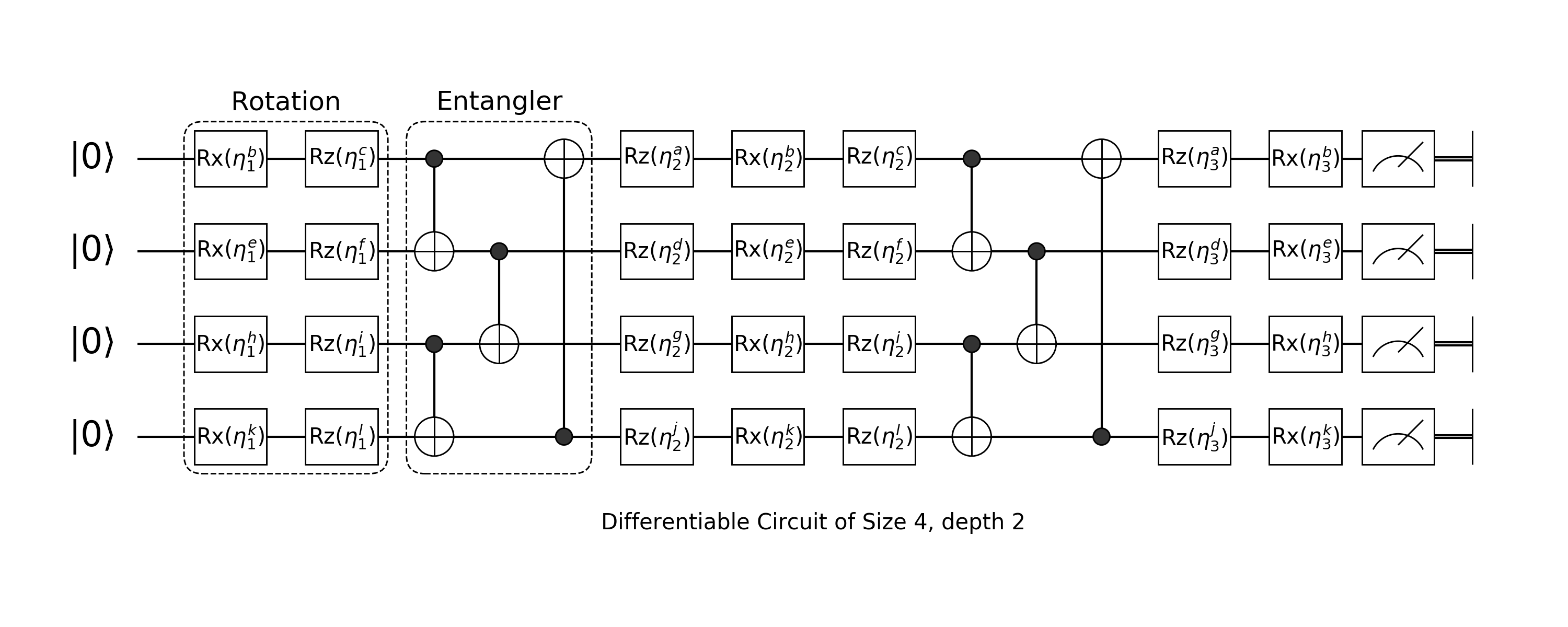
It is composited by two different layers: rotation layer and entangler layer.

Rotation Layer

Arbitrary rotation is built with Rotation Gate on Z, X, Z axis with parameters.

\[Rz(\theta) \cdot Rx(\theta) \cdot Rz(\theta)\]

Since our input will be a $|0\dots 0\rangle$ state. The first layer of arbitrary rotation can just use $Rx(\theta) \cdot Rz(\theta)$ and the last layer of arbitrary rotation could just use $Rz(\theta)\cdot Rx(\theta)$

In 幺, every Hilbert operator is a block type, this ncludes all quantum gates and quantum oracles. In general, operators appears in a quantum circuit can be divided into Composite Blocks and Primitive Blocks.

We follow the low abstraction principle and thus each block represents a certain approach of calculation. The simplest Composite Block is a Chain Block, which chains other blocks (oracles) with the same number of qubits together. It is just a simple mathematical composition of operators with same size. e.g.

\[\text{chain(X, Y, Z)} \iff X \cdot Y \cdot Z\]

We can construct an arbitrary rotation block by chain $Rz$, $Rx$, $Rz$ together.

chain(Rz(0.0), Rx(0.0), Rz(0.0))

nqubits: 1
chain
├─ rot(Z, 0.0)
├─ rot(X, 0.0)
└─ rot(Z, 0.0)

Rx, Rz will construct new rotation gate, which are just shorthands for rot(X, 0.0), etc.

Then let's chain them up

layer(nbit::Int, x::Symbol) = layer(nbit, Val(x))
layer(nbit::Int, ::Val{:first}) = chain(nbit, put(i=>chain(Rx(0), Rz(0))) for i = 1:nbit);

We do not need to feed the first n parameter into put here. All factory methods can be lazy evaluate the first arguements, which is the number of qubits. It will return a lambda function that requires a single interger input. The instance of desired block will only be constructed until all the information is filled. When you filled all the information in somewhere of the declaration, 幺 will be able to infer the others. We will now define the rest of rotation layers

layer(nbit::Int, ::Val{:last}) = chain(nbit, put(i=>chain(Rz(0), Rx(0))) for i = 1:nbit)
layer(nbit::Int, ::Val{:mid}) = chain(nbit, put(i=>chain(Rz(0), Rx(0), Rz(0))) for i = 1:nbit);

Entangler

Another component of quantum circuit born machine are several CNOT operators applied on different qubits.

entangler(pairs) = chain(control(ctrl, target=>X) for (ctrl, target) in pairs);

We can then define such a born machine

function build_circuit(n, nlayers, pairs)
    circuit = chain(n)
    push!(circuit, layer(n, :first))
    for i in 2:nlayers
        push!(circuit, cache(entangler(pairs)))
        push!(circuit, layer(n, :mid))
    end
    push!(circuit, cache(entangler(pairs)))
    push!(circuit, layer(n, :last))
    return circuit
end

build_circuit (generic function with 1 method)

We use the method cache here to tag the entangler block that it should be cached after its first run, because it is actually a constant oracle. Let's see what will be constructed

build_circuit(4, 1, [1=>2, 2=>3, 3=>4])

nqubits: 4
chain
├─ chain
│  ├─ put on (1)
│  │  └─ chain
│  │     ├─ rot(X, 0.0)
│  │     └─ rot(Z, 0.0)
│  ├─ put on (2)
│  │  └─ chain
│  │     ├─ rot(X, 0.0)
│  │     └─ rot(Z, 0.0)
│  ├─ put on (3)
│  │  └─ chain
│  │     ├─ rot(X, 0.0)
│  │     └─ rot(Z, 0.0)
│  └─ put on (4)
│     └─ chain
│        ├─ rot(X, 0.0)
│        └─ rot(Z, 0.0)
├─ [cached] chain
│     ├─ control(1)
│     │  └─ (2,) X
│     ├─ control(2)
│     │  └─ (3,) X
│     └─ control(3)
│        └─ (4,) X
└─ chain
   ├─ put on (1)
   │  └─ chain
   │     ├─ rot(Z, 0.0)
   │     └─ rot(X, 0.0)
   ├─ put on (2)
   │  └─ chain
   │     ├─ rot(Z, 0.0)
   │     └─ rot(X, 0.0)
   ├─ put on (3)
   │  └─ chain
   │     ├─ rot(Z, 0.0)
   │     └─ rot(X, 0.0)
   └─ put on (4)
      └─ chain
         ├─ rot(Z, 0.0)
         └─ rot(X, 0.0)

MMD Loss & Gradients

The MMD loss is describe below:

\[\begin{aligned} \mathcal{L} &= \left| \sum_{x} p \theta(x) \phi(x) - \sum_{x} \pi(x) \phi(x) \right|^2\\ &= \langle K(x, y) \rangle_{x \sim p_{\theta}, y\sim p_{\theta}} - 2 \langle K(x, y) \rangle_{x\sim p_{\theta}, y\sim \pi} + \langle K(x, y) \rangle_{x\sim\pi, y\sim\pi} \end{aligned}\]

We will use a squared exponential kernel here.

struct RBFKernel
    σ::Float64
    m::Matrix{Float64}
end

function RBFKernel(σ::Float64, space)
    dx2 = (space .- space').^2
    return RBFKernel(σ, exp.(-1/2σ * dx2))
end

kexpect(κ::RBFKernel, x, y) = x' * κ.m * y

kexpect (generic function with 1 method)

There are two different way to define the loss:

In simulation we can use the probability distribution of the state directly

get_prob(qcbm) = probs(zero_state(nqubits(qcbm)) |> qcbm)

function loss(κ, c, target)
    p = get_prob(c) - target
    return kexpect(κ, p, p)
end

loss (generic function with 1 method)

Or if you want to simulate the whole process with measurement (which is entirely physical), you should define the loss with measurement results, for convenience we directly use the simulated results as our loss

Gradients

the gradient of MMD loss is

\[\begin{aligned} \frac{\partial \mathcal{L}}{\partial \theta^i_l} &= \langle K(x, y) \rangle_{x\sim p_{\theta^+}, y\sim p_{\theta}} - \langle K(x, y) \rangle_{x\sim p_{\theta}^-, y\sim p_{\theta}}\\ &- \langle K(x, y) \rangle _{x\sim p_{\theta^+}, y\sim\pi} + \langle K(x, y) \rangle_{x\sim p_{\theta^-}, y\sim\pi} \end{aligned}\]

which can be implemented as

function gradient(qcbm, κ, ptrain)
    n = nqubits(qcbm)
    prob = get_prob(qcbm)
    grad = zeros(Float64, nparameters(qcbm))

    count = 1
    for k in 1:2:length(qcbm), each_line in qcbm[k], gate in content(each_line)
        dispatch!(+, gate, π/2)
        prob_pos = probs(zero_state(n) |> qcbm)

        dispatch!(-, gate, π)
        prob_neg = probs(zero_state(n) |> qcbm)

        dispatch!(+, gate, π/2) # set back

        grad_pos = kexpect(κ, prob, prob_pos) - kexpect(κ, prob, prob_neg)
        grad_neg = kexpect(κ, ptrain, prob_pos) - kexpect(κ, ptrain, prob_neg)
        grad[count] = grad_pos - grad_neg
        count += 1
    end
    return grad
end

gradient (generic function with 1 method)

Now let's setup the training

import Optimisers
qcbm = build_circuit(6, 10, [1=>2, 3=>4, 5=>6, 2=>3, 4=>5, 6=>1])
dispatch!(qcbm, :random) # initialize the parameters

κ = RBFKernel(0.25, 0:2^6-1)
pg = gaussian_pdf(1:1<<6, 1<<5-0.5, 1<<4);
opt = Optimisers.setup(Optimisers.ADAM(0.01), parameters(qcbm));

function train(qcbm, κ, opt, target)
    history = Float64[]
    for _ in 1:100
        push!(history, loss(κ, qcbm, target))
        ps = parameters(qcbm)
        Optimisers.update!(opt, ps, gradient(qcbm, κ, target))
        dispatch!(qcbm, ps)
    end
    return history
end

history = train(qcbm, κ, opt, pg)
trained_pg = probs(zero_state(nqubits(qcbm)) |> qcbm)

64-element Vector{Float64}:
 0.00438976398103501
 0.004789811770827422
 0.005469407177785036
 0.005846628409164073
 0.0067423476264781455
 0.007278111131594668
 0.008088969094080255
 0.008903991247850086
 0.009766502605001691
 0.010549704518680307
 0.011485543748993387
 0.012449565215968822
 0.013415707718422
 0.014372119872537033
 0.01533765071638782
 0.01643684247899615
 0.017300692522607096
 0.01838175164331962
 0.01916348822960736
 0.020293352558245298
 0.020987430831875244
 0.02186513791391436
 0.022656535057094942
 0.02333217574469658
 0.024134408657782824
 0.024731362064557182
 0.02505899757712401
 0.02558906668117212
 0.0258402609669878
 0.026022479471334896
 0.026137077796875026
 0.0260377314560077
 0.026066725230865295
 0.02574463279556061
 0.025583705211262513
 0.02498578577117489
 0.024642859980917708
 0.023976364921269054
 0.023533298665565472
 0.02261893291105684
 0.021981745618188334
 0.02109029440287281
 0.020231860087169398
 0.019252071324016753
 0.018211469426893848
 0.017391466098259693
 0.0163510262791668
 0.015355894429129461
 0.014143934286302931
 0.013382304780344667
 0.01228725260588839
 0.01156953805260446
 0.010561739960596655
 0.00967591539712026
 0.009050827006924195
 0.008130377734940962
 0.007146791804454289
 0.00651318493013978
 0.006147399312632998
 0.00529678988471932
 0.004716790314173247
 0.004219311603692107
 0.0038085492649044704
 0.003476543420185151

The history of training looks like below

title!("training history")
xlabel!("steps"); ylabel!("loss")
plot(history)

And let's check what we got

fig2 = plot(1:1<<6, trained_pg; label="trained")
plot!(fig2, 1:1<<6, pg; label="target")
title!("distribution")
xlabel!("x"); ylabel!("p")

So within 50 steps, we got a pretty close estimation of our target distribution!

This page was generated using Literate.jl.