Quantum Circuit Born Machine

Reference: Jin-Guo Liu, Lei Wang (2018) Differentiable Learning of Quantum Circuit Born Machine

using Yao, Yao.Blocks
using LinearAlgebra

Training target

A gaussian distribution

\[f(x \left| \mu, \sigma^2\right) = \frac{1}{\sqrt{2\pi\sigma^2}} e^{-\frac{(x-\mu)^2}{2\sigma^2}}\]

function gaussian_pdf(x, μ::Real, σ::Real)
    pl = @. 1 / sqrt(2pi * σ^2) * exp(-(x - μ)^2 / (2 * σ^2))
    pl / sum(pl)
end
pg = gaussian_pdf(1:1<<6, 1<<5-0.5, 1<<4);

This distribution looks like Gaussian Distribution

Build Circuits

Building Blocks

Gates are grouped to become a layer in a circuit, this layer can be Arbitrary Rotation or CNOT entangler. Which are used as our basic building blocks of Born Machines.

differentiable ciruit

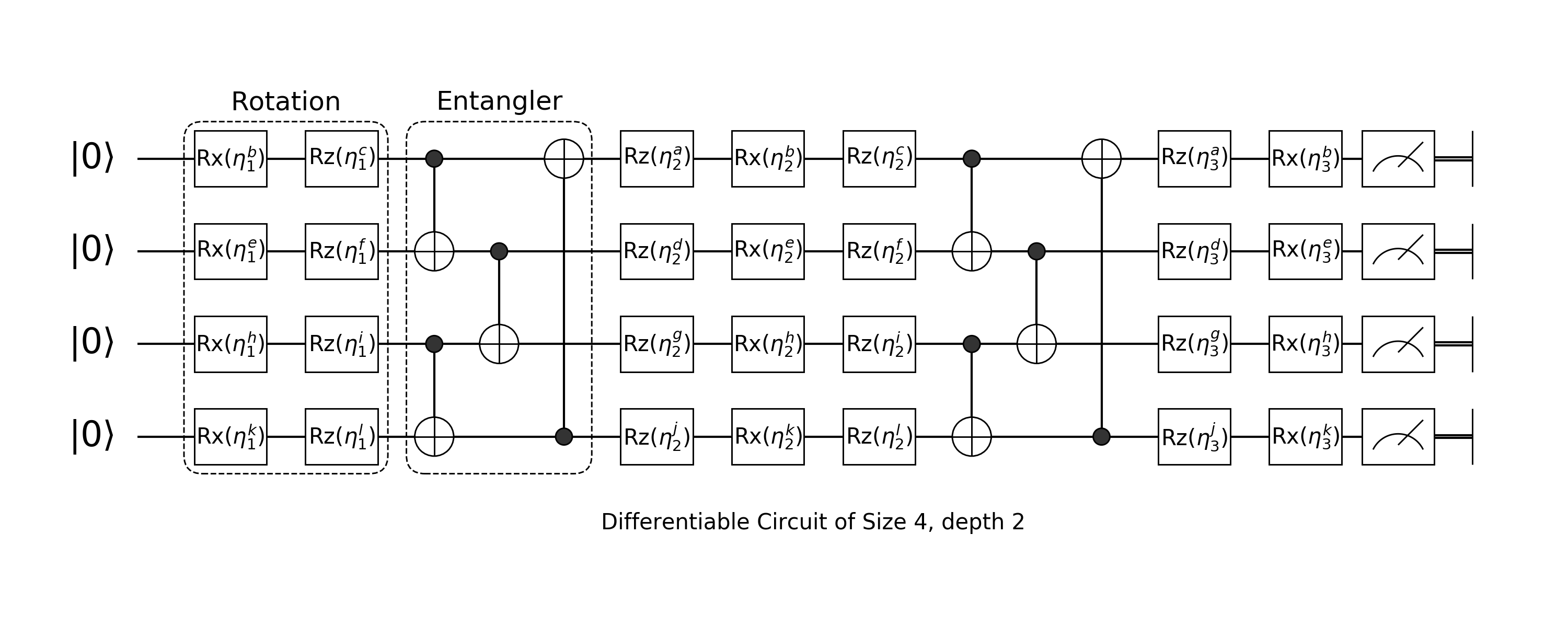
Arbitrary Rotation

Arbitrary Rotation is built with Rotation Gate on Z, Rotation Gate on X and Rotation Gate on Z:

\[Rz(\theta) \cdot Rx(\theta) \cdot Rz(\theta)\]

Since our input will be a $|0\dots 0\rangle$ state. The first layer of arbitrary rotation can just use $Rx(\theta) \cdot Rz(\theta)$ and the last layer of arbitrary rotation could just use $Rz(\theta)\cdot Rx(\theta)$

In 幺, every Hilbert operator is a block type, this includes all quantum gates and quantum oracles. In general, operators appears in a quantum circuit can be divided into Composite Blocks and Primitive Blocks.

We follow the low abstraction principle and thus each block represents a certain approach of calculation. The simplest Composite Block is a Chain Block, which chains other blocks (oracles) with the same number of qubits together. It is just a simple mathematical composition of operators with same size. e.g.

\[\text{chain(X, Y, Z)} \iff X \cdot Y \cdot Z\]

We can construct an arbitrary rotation block by chain $Rz$, $Rx$, $Rz$ together.

chain(Rz(0), Rx(0), Rz(0))

Total: 1, DataType: Complex{Float64}
chain
├─ Rot Z gate: 0.0
├─ Rot X gate: 0.0
└─ Rot Z gate: 0.0

Rx, Ry and Rz will construct new rotation gate, which are just shorthands for rot(X, 0.0), etc.

Then, let's chain them up

layer(nbit::Int, x::Symbol) = layer(nbit, Val(x))
layer(nbit::Int, ::Val{:first}) = chain(nbit, put(i=>chain(Rx(0), Rz(0))) for i = 1:nbit);

Here, we do not need to feed the first nbit parameter into put. All factory methods can be lazy evaluate the first arguements, which is the number of qubits. It will return a lambda function that requires a single interger input. The instance of desired block will only be constructed until all the information is filled. When you filled all the information in somewhere of the declaration, 幺 will be able to infer the others. We will now define the rest of rotation layers

layer(nbit::Int, ::Val{:last}) = chain(nbit, put(i=>chain(Rz(0), Rx(0))) for i = 1:nbit)
layer(nbit::Int, ::Val{:mid}) = chain(nbit, put(i=>chain(Rz(0), Rx(0), Rz(0))) for i = 1:nbit);

CNOT Entangler

Another component of quantum circuit born machine is several CNOT operators applied on different qubits.

entangler(pairs) = chain(control([ctrl, ], target=>X) for (ctrl, target) in pairs);

We can then define such a born machine

function build_circuit(n::Int, nlayer::Int, pairs)
    circuit = chain(n)
    push!(circuit, layer(n, :first))

    for i = 1:(nlayer - 1)
        push!(circuit, cache(entangler(pairs)))
        push!(circuit, layer(n, :mid))
    end

    push!(circuit, cache(entangler(pairs)))
    push!(circuit, layer(n, :last))

    circuit
end;

We use the method cache here to tag the entangler block that it should be cached after its first run, because it is actually a constant oracle. Let's see what will be constructed

julia> build_circuit(4, 1, [1=>2, 2=>3, 3=>4]) |> autodiff(:QC)
Total: 4, DataType: Complex{Float64}
chain
├─ chain
│  ├─ put on (1)
│  │  └─ chain
│  │     ├─ [̂∂] Rot X gate: 0.0
│  │     └─ [̂∂] Rot Z gate: 0.0
│  ├─ put on (2)
│  │  └─ chain
│  │     ├─ [̂∂] Rot X gate: 0.0
│  │     └─ [̂∂] Rot Z gate: 0.0
│  ├─ put on (3)
│  │  └─ chain
│  │     ├─ [̂∂] Rot X gate: 0.0
│  │     └─ [̂∂] Rot Z gate: 0.0
│  └─ put on (4)
│     └─ chain
│        ├─ [̂∂] Rot X gate: 0.0
│        └─ [̂∂] Rot Z gate: 0.0
├─ [↺] chain
│  ├─ control(1)
│  │  └─ (2,)=>X gate
│  ├─ control(2)
│  │  └─ (3,)=>X gate
│  └─ control(3)
│     └─ (4,)=>X gate
└─ chain
   ├─ put on (1)
   │  └─ chain
   │     ├─ [̂∂] Rot Z gate: 0.0
   │     └─ [̂∂] Rot X gate: 0.0
   ├─ put on (2)
   │  └─ chain
   │     ├─ [̂∂] Rot Z gate: 0.0
   │     └─ [̂∂] Rot X gate: 0.0
   ├─ put on (3)
   │  └─ chain
   │     ├─ [̂∂] Rot Z gate: 0.0
   │     └─ [̂∂] Rot X gate: 0.0
   └─ put on (4)
      └─ chain
         ├─ [̂∂] Rot Z gate: 0.0
         └─ [̂∂] Rot X gate: 0.0

RotationGates inside this circuit are automatically marked by [̂∂], which means parameters inside are diferentiable. autodiff has two modes, one is autodiff(:QC), which means quantum differentiation with simulation complexity $O(M^2)$ ($M$ is the number of parameters), the other is classical backpropagation autodiff(:BP) with simulation coplexity $O(M)$.

Let's define a circuit to use later

circuit = build_circuit(6, 10, [1=>2, 3=>4, 5=>6, 2=>3, 4=>5, 6=>1]) |> autodiff(:QC)
dispatch!(circuit, :random);

Here, the function autodiff(:QC) will mark rotation gates in a circuit as differentiable automatically.

MMD Loss & Gradients

The MMD loss is describe below:

\[\begin{aligned} \mathcal{L} &= \left| \sum_{x} p \theta(x) \phi(x) - \sum_{x} \pi(x) \phi(x) \right|^2\\ &= \langle K(x, y) \rangle_{x \sim p_{\theta}, y\sim p_{\theta}} - 2 \langle K(x, y) \rangle_{x\sim p_{\theta}, y\sim \pi} + \langle K(x, y) \rangle_{x\sim\pi, y\sim\pi} \end{aligned}\]

We will use a squared exponential kernel here.

struct RBFKernel
    sigma::Float64
    matrix::Matrix{Float64}
end

"""get kernel matrix"""
kmat(mbf::RBFKernel) = mbf.matrix

"""statistic functional for kernel matrix"""
kernel_expect(kernel::RBFKernel, px::Vector, py::Vector=px) = px' * kmat(kernel) * py;

Now let's define the RBF kernel matrix used in calculation

function rbf_kernel(basis, σ::Real)
    dx2 = (basis .- basis').^2
    RBFKernel(σ, exp.(-1/2σ * dx2))
end

kernel = rbf_kernel(0:1<<6-1, 0.25);

Next, we build a QCBM setup, which is a combination of circuit, kernel and target probability distribution ptrain Its loss function is MMD loss, if and only if it is 0, the output probability of circuit matches ptrain exactly.

struct QCBM{BT<:AbstractBlock}
    circuit::BT
    kernel::RBFKernel
    ptrain::Vector{Float64}
end

"""get wave function"""
psi(qcbm::QCBM) = zero_state(qcbm.circuit |> nqubits) |> qcbm.circuit

"""extract probability dierctly"""
Yao.probs(qcbm::QCBM) = qcbm |> psi |> probs

"""the loss function"""
function mmd_loss(qcbm, p=qcbm|>probs)
    p = p - qcbm.ptrain
    kernel_expect(qcbm.kernel, p, p)
end;

problem setup

qcbm = QCBM(circuit, kernel, pg);

Gradients

the gradient of MMD loss is

\[\begin{aligned} \frac{\partial \mathcal{L}}{\partial \theta^i_l} &= \langle K(x, y) \rangle_{x\sim p_{\theta^+}, y\sim p_{\theta}} - \langle K(x, y) \rangle_{x\sim p_{\theta}^-, y\sim p_{\theta}}\\ &- \langle K(x, y) \rangle _{x\sim p_{\theta^+}, y\sim\pi} + \langle K(x, y) \rangle_{x\sim p_{\theta^-}, y\sim\pi} \end{aligned}\]

function mmdgrad(qcbm::QCBM, dbs; p0::Vector)
    statdiff(()->probs(qcbm) |> as_weights, dbs, StatFunctional(kmat(qcbm.kernel)), initial=p0 |> as_weights) -
        2*statdiff(()->probs(qcbm) |> as_weights, dbs, StatFunctional(kmat(qcbm.kernel)*qcbm.ptrain))
end;

Optimizer

We will use the Adam optimizer. Since we don't want you to install another package for this, the following code for this optimizer is copied from Knet.jl

Reference: Kingma, D. P., & Ba, J. L. (2015). Adam: a Method for Stochastic Optimization. International Conference on Learning Representations, 1–13.

mutable struct Adam
    lr::AbstractFloat
    gclip::AbstractFloat
    beta1::AbstractFloat
    beta2::AbstractFloat
    eps::AbstractFloat
    t::Int
    fstm
    scndm
end

Adam(; lr=0.001, gclip=0, beta1=0.9, beta2=0.999, eps=1e-8)=Adam(lr, gclip, beta1, beta2, eps, 0, nothing, nothing)

function update!(w, g, p::Adam)
    gclip!(g, p.gclip)
    if p.fstm===nothing; p.fstm=zero(w); p.scndm=zero(w); end
    p.t += 1
    lmul!(p.beta1, p.fstm)
    BLAS.axpy!(1-p.beta1, g, p.fstm)
    lmul!(p.beta2, p.scndm)
    BLAS.axpy!(1-p.beta2, g .* g, p.scndm)
    fstm_corrected = p.fstm / (1 - p.beta1 ^ p.t)
    scndm_corrected = p.scndm / (1 - p.beta2 ^ p.t)
    BLAS.axpy!(-p.lr, @.(fstm_corrected / (sqrt(scndm_corrected) + p.eps)), w)
end

function gclip!(g, gclip)
    if gclip == 0
        g
    else
        gnorm = vecnorm(g)
        if gnorm <= gclip
            g
        else
            BLAS.scale!(gclip/gnorm, g)
        end
    end
end
optim = Adam(lr=0.1);

Start Training

We define an iterator called QCBMOptimizer. We want to realize some interface like

for x in qo
    # runtime result analysis
end

Although such design makes the code a bit more complicated, but one will benefit from this interfaces when doing run time analysis, like keeping track of the loss.

struct QCBMOptimizer
    qcbm::QCBM
    optimizer
    dbs
    params::Vector
    QCBMOptimizer(qcbm::QCBM, optimizer) = new(qcbm, optimizer, collect(qcbm.circuit, AbstractDiff), parameters(qcbm.circuit))
end

In the initialization of QCBMOptimizer instance, we collect all differentiable units into a sequence dbs for furture use.

iterator interface To support iteration operations, Base.iterate should be implemented

function Base.iterate(qo::QCBMOptimizer, state::Int=1)
    p0 = qo.qcbm |> probs
    grad = mmdgrad.(Ref(qo.qcbm), qo.dbs, p0=p0)
    update!(qo.params, grad, qo.optimizer)
    dispatch!(qo.qcbm.circuit, qo.params)
    (p0, state+1)
end

In each iteration, the iterator will return the generated probability distribution in current step. During each iteration step, we broadcast mmdgrad function over dbs to obtain all gradients. Here, To avoid the QCBM instance from being broadcasted, we wrap it with Ref to create a reference for it. The training of the quantum circuit is simple, just iterate through the steps.

history = Float64[]
for (k, p) in enumerate(QCBMOptimizer(qcbm, optim))
    curr_loss = mmd_loss(qcbm, p)
    push!(history, curr_loss)
    k%5 == 0 && println("k = ", k, " loss = ", curr_loss)
    k >= 50 && break
end

k = 5 loss = 0.00847749636271937
k = 10 loss = 0.0022075107632702835
k = 15 loss = 0.0013664488262862158
k = 20 loss = 0.0008221894171723352
k = 25 loss = 0.0004509647774503069
k = 30 loss = 0.0002799245762106908
k = 35 loss = 0.0001433244922560841
k = 40 loss = 9.266614925835051e-5
k = 45 loss = 4.383088287793888e-5
k = 50 loss = 3.559024250813189e-5

The training history looks like History

and the learnt distribution

This page was generated using Literate.jl.